Overfitting or Underfitting? Bias-Variance Trade Off From Learning Curve

What is bias, variance? How to interpret learning curve? How do we diagnose bias and variance? And, what should we do to deal with it?

Introduction

In supervised learning, we have target variables provided to be compared with prediction for judging model performance. We assume there is a unknown model, f, that best describe the data, our task is to find the estimate of f. The main sources of learning error in a model is noise, bias, and variance. Noise is irreducible by the learning process .Our goal is always to build a model with good generalization capability beyond training data.

Is oversized good? (from disneyclips.com)

Bias-Variance

Bias evaluates model learning ability, computing difference between true values and predicted values. Under most circumstance, we try to make some assumption about the model, for example, when applying linear regression, we assume input and output have linear relationship. Often the relationship n real world problem is non-linear, model estimated does not fit data well. The erroneous assumption leads to high bias. Conversely, if model estimated fit data too well, and it captures almost all the difference, including noise, it results low bias.

• High bias — Model outputs are too far away from true values. Poor performance on training and test datasets.
• Low bias — Good performance on training datasets.

Variance quantifies variability of model results when a new set of data obtained from same process as training data, is input into the model. As mentioned in introduction, we aim to find a good estimate of f, we obtain a different estimates when we use different sets of data from same population. Variance determines how much the estimates of f vary.

• Variance is high when the training error is low, but test error is high.

Low bias, high variance.

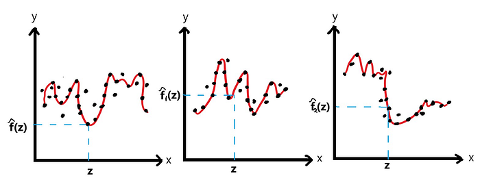
From the plots above, estimates of f fits every dat points almost perfectly for each set of data, hence low bias. Apparently, the fitted lines differ significantly. However, when prediction for a particular point with fitted line varies. This implies high variance. When we have a situation where the lines are oversimplified, we will encounter reversed results. High bias, low variance.

High bias, low variance.

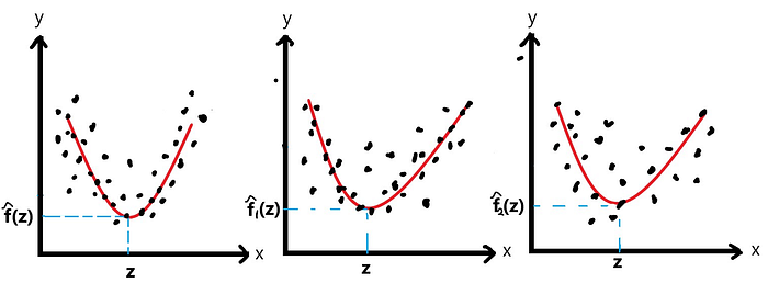
Due to the reasoning above, we want low bias, low variance. Nevertheless, in practice, there might be noise when we collect the data, such as sampling noise which cannot be improved by a good model. An extremely low bias model may have captures all these sources of errors in training data, resulting poor performance on test data or out-of-sample data (a set of data that we set aside until the best model is built, then test is done on it).

• When we make prediction, it can be higher or lower than true value, their difference can be positive or negative, there is possibility of eliminating total bias. Therefore we tend to compute and visualize bias squared.
• Bias squared decreases exponentially with model complexity.
• Variance increases exponentially with model complexity.
• Irreducible error, such as random noise in sampling process, will be remained constant, unaffected by model complexity.

There is conflict when we try to minimize these two types of errors simultaneously. Bias increase when variance decreases, and vice versa. Bias-variance trade-off idea arises, we are looking for the balance point between bias and variance, neither oversimply nor overcomplicate the model estimates.

• Low bias, low variance: Good model.
• High bias, low variance: Oversimplify the model, it does not capture information from data and producing poor prediction. Underfitting happened.
• Low bias, high variance — Overcomplicate model. It performs well for training dataset but poor for test dataset. It captures the random noise present in training data, does not generalize to unseen data.

Learning Curve

Learning curve is a plot of error against size of training data. for this section, we are dividing data into training and validation data sets. Let’s take two extreme points in the plot below to explore the idea.

Curve with different Biases.

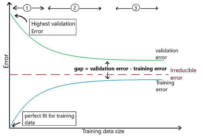
1. When model fits only a single data point, fitted line is exactly on the data point and hence zero training error. But, when it is applied to unseen validation data, it gives a high validation error.
2. When size of training instances increases, the fitted line is minimizing error over all data points, it will not fit all data perfectly. It tends to lie in between the points. It capture useful information, and reducing the impact of noise. Hence, training error increases, validation error decreases.
3. The optimal training data size is the point where the curves become plateau beyond it. Increasing size further will just reduce the efficiency of training process, without any improvement. Increasing size of training data does not help if the curves are stagnant.

How to determine the bias and variance from learning curve?

Curve with different Biases.

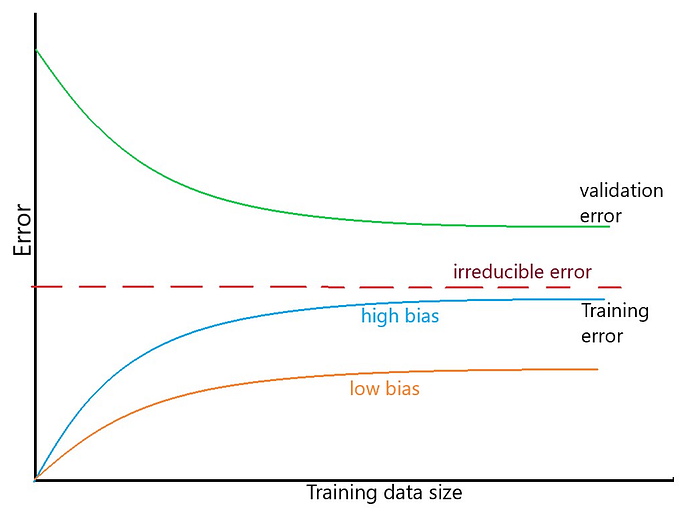
As discussed, the error reading of training curve gives information about bias. Low training error means low bias, and vice versa. Training error increases and validation error decreases as the training data size increases. The model starts to capture more useful information from training data and generalize better. Next question, how is variance examined? This is pretty straight forward. The gap between training and validation curves answers the question. The narrower the gap, the lower the variance, vice versa.

Size of gap = variance.

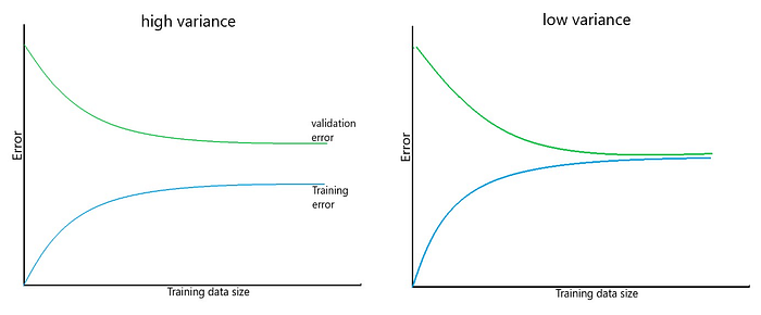
Suggestion to consider to deal with bias and variance problem.

High bias, low variance — Underfitting:

• It is mostly useless to increase training instances. The model does not even fit current set of data good enough.
• Increase model complexity by decreasing regularization OR increasing dimension of features input.

Low bias, high variance — Overfitting:

• Increase training instances — The model fits current set of training data well, exposure to mode data points might reveal extra knowledge to the learner and become more generalized.
• Decrease model complexity by increase regularization OR features selection (reducing features frame dimension)

KNN is the most typical machine learning model used to explain bias-variance trade-off idea. When we have a small k, we have a rather complex model with low bias and high variance. For example, when we have k=1, we simply predict according to nearest point. As k increases, we are averaging the labels of k nearest points. Hence, bias increases and variances decreases.

Conclusion

Bias-variance trade-off can be a good starting point to understand about overfitting and underfitting phenomenon, which are the main concern or ultimate goal in model training process, seeking for optimal model that generalized well.